About the NCEA network appraisal tool
Natural Capital and Ecosystem Assessment (NCEA) is a science innovation and transformation programme, which spans across land and water environments. It has been set up to collect data on the extent, condition and change over time of England's ecosystems and natural capital, and the benefits to society. This Network Appraisal Tool has been developed as part of the Environment Agency's NCEA Water Quantity Monitoring project. For more information about the project please contact: NCEAprogramme@environment-agency.gov.uk.
The NCEA Network Appraisal Tool is designed to be intuitive, with dropdowns and graph formats from which to select, and tool tips providing definitions of metadata parameters. The tool enables users to explore metadata associated with river flow monitoring sites (gauging stations) and to visualise how representative a selected set of monitoring sites are of river catchments across England. These user notes are provided to assist with getting started, and are thus concise, with the focus on basic functionality.
How to use the portal
How to edit the map display
- Zooming in and out is possible using the + and - buttons or the mouse wheel
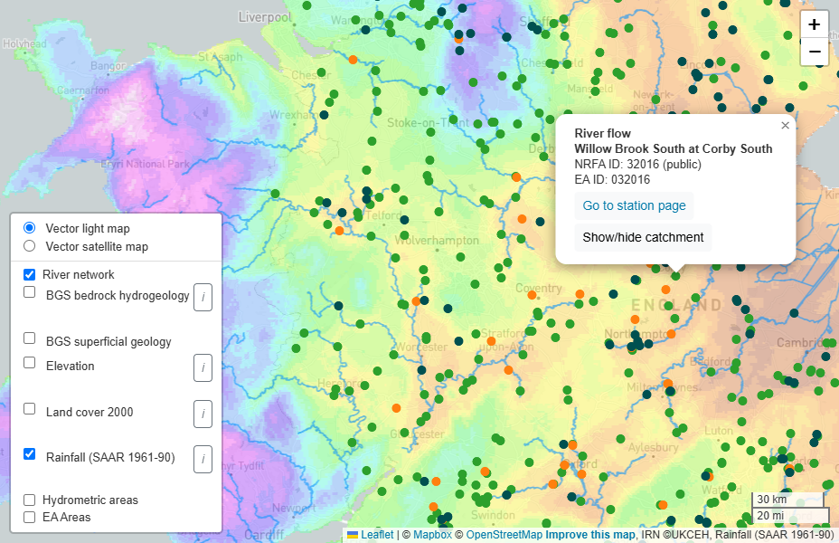
- The map can be displayed in vector format. Vector maps are high quality images suitable for reproduction in a report (by snipping or screenshot)
- Panning is possible using the hand icon
- Information (satellite image, river network, hydrometric areas, EA Areas) can be added to the map or removed via the layer icon (at the bottom left of the map)
- Spatial data can be added when sufficiently zoomed in (bedrock hydrogeology, superficial geology, elevation, land cover and rainfall).
- Station catchment polygons are available to view on the map for public NRFA stations only (use NRFA public symbology). Click on an NRFA public station on the map to view its popup, which has the Show/hide catchment button.
How to filter catchments
- Filters are provided for a large suite of metadata parameters as dropdowns under the following categories:
- Basic (including Location, EA Area, Record length)
- NRFA data types (Peak flow, Daily flow, Live data)
- Location (including Easting, Northing and Station level)
- Category (FEH Suitability)
- Station information (Station type, Sensitivity, Co-located index sites and Co-located with)
- Catchment information (including Factors affecting runoff)
- Daily flow statistics (including FDC statistics, Completeness, base flow index)
- Peak flow statistics (including QMED, Peak flow start date)
- Elevation (Min, Max and 10th, 50th and 90th centiles)
- Catchment rainfall (SAAR4170, SAAR6190, SAAR8110)
- Land cover (Arable/horticultural, Grassland, Mountain/heath/bog, Woodland, Urban)
- Geology (high/moderate/low permeability bedrock, high/low/mixed permeability superficial deposits)
- FEH Descriptors (including BFIHOST and FARL)
- Sub-networks (including UK Benchmark, etc)
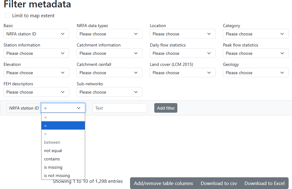
- Having selected the parameter, select a range/condition to apply via the dropdown box (e.g between, is missing), and then “Add filter”
- Multiple filters can be added to build a query, and any of these removed using the “x” next to the filter (e.g. GSDQ overall class = G, Figure 2).
How to use the co-location filter
- At some locations, there are two or more gauging stations, for example, because different instruments, structures or replacement stations are held under different station numbers. Catchment information for such co-located sites may be duplicated, introducing a slight bias. To resolve this, a 'co-location index' is used to identify one of the sites at each location
- When assessing the monitoring at a location, no filtering of this index is required
- When assessing representativeness, the user may wish to remove the resulting duplication of the catchments and their spatial data by filtering 'Co-location index = TRUE'. They can also be included or excluded from graphs and statistics using the toggle switch provided
- Note that the selection of the index site at each location is arbitrary, and does not indicate a primary site at the location. The co-located sites may be investigated using the 'Co-located with' attribute
How to edit and download the metadata table
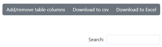
- Columns displayed in the table under the map can be added and removed via the
 button, and columns are automatically added when selected as a filter
 - Each catchment/gauging station meeting the current filter criteria has a row in the table. The table will update whenever the filter criteria are changed, and the number of catchments meeting the filter criteria is shown above the table
- The table can be sorted by any column by double clicking on the column heading
- The table is searchable and can be downloaded using the controls above the header row
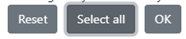
- To download all available metadata for all catchments/gauging stations, use the 'Select all' button at the bottom of the column selection window, and remove any filters before downloading to csv
How to add symbology
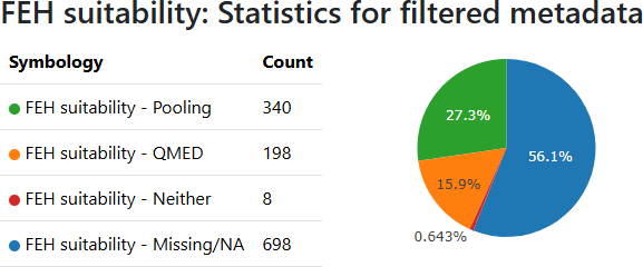
- Using the dropdown at the top of the Network Appraisal Tool, select a parameter that will be used to categorise/classify the metadata, and colour code the map and graphics.
- Parameters available for symbology are categorical rather than numerical, such as FEH Suitability and NRFA data type
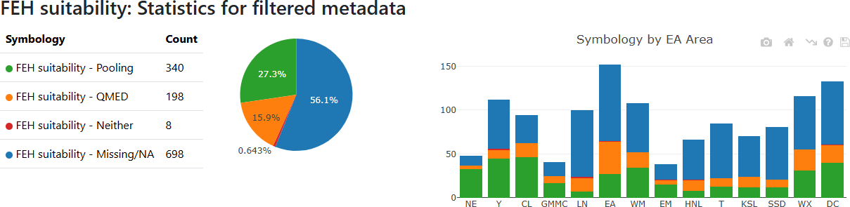
- When any parameter is selected for symbology, graphics beneath the main metadata table show the numbers of catchments/gauging stations in each category/class for the whole table.
How to manipulate and export histograms
- Under the metadata table, select a parameter to plot as a histogram for the filtered catchments/gauging stations
- To toggle between the histogram and cumulative distribution plot, using the 'Cumulative' tick box above the plot
- Pop up information is available on each bar of the histogram by hovering over it
- Further options are available by hovering at the top right corner of the plot, including the download of the bins and distributions as a .csv file
- All plots are zoomable, by dragging and releasing the left mouse button. To return to the original settings, double click on the plot, or use the 'reset axes' button.
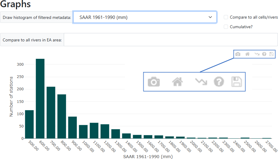
Icons, left to right:
- download plot as .png
- reset axes
- linear or log scale toggle
- toggle legend (on/off)
- download data as csv
How to manipulate and export scatter plots
- Having plotted a histogram of a selected parameter (x), select a second parameter (y) to generate the scatter plot from the dropdown 'Draw scatter plot of (x) vs (y)'
- A third parameter (z) can be added to generate a three dimensional scatter plot using the 'Add to scatter plot (z)' dropdown. This can be rotated to visualise the relationships between the three parameters from any angle
- The same plotting options are available as for the histograms, plus the additional functionality of hovering over points to identify individual catchments/gauging stations
- Additional plotting options are available, to the top right of the 3D scatter plot
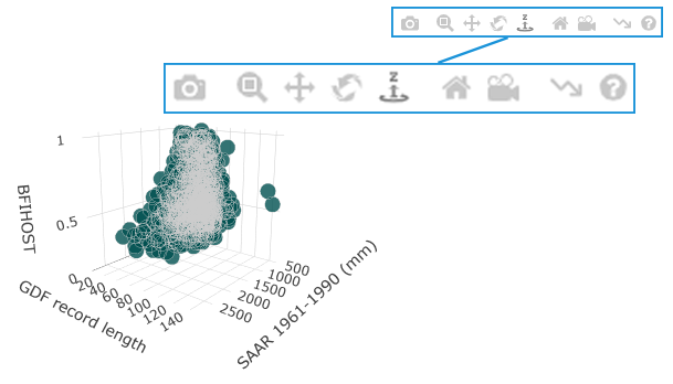
Icons, left to right:
- download plot as .png
- zoom
- pan
- orbital rotation
- turntable rotation
- reset camera to default
- reset camera to last save
- linear or log scale toggle
- toggle legend (on/off)
How to assess representativeness
Once a histogram has been plotted, the distribution of a parameter for a subset of filtered gauging station catchments can be compared to that of all river catchments in England by clicking the 'Compare to all England rivers (all cells)' tickbox above the histogram
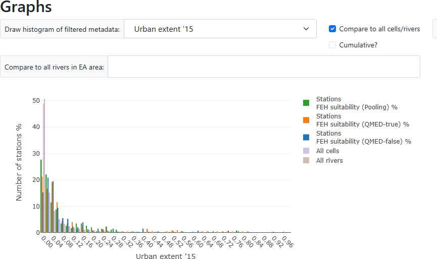
As for a single histogram the 'Cumulative' tickbox' can be used to toggle between histogram and cumulative distribution plots, and both the plot and underlying data are downloadable
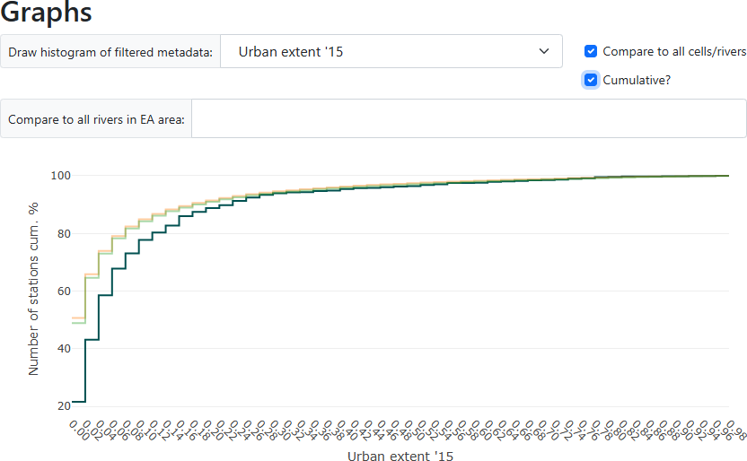
This functionality is available for catchment area, rainfall (SAAR), all five land cover types and all 21 FEH catchment descriptors (such as BFIHOST and FARL)
How to compare Environment Agency areas
- To filter the catchments/gauging stations for a single EA Area of interest, select 'EA Area' from the Basic category, and select the Area from the list
- To explore the representativeness of the Area's gauged catchments, use the 'Compare to all England rivers (all cells) in EA Area:' dropdown
- To allow comparison of all river catchments between EA Areas, multiple Areas can be selected in the 'Compare to all England rivers (all cells) in EA Area' box
- When any parameter is selected for symbology, the graphics beneath the main metadata table show the numbers of catchments/gauging stations in each category/class for the whole table (as shown in 'How to add symbology' above), and also broken down by EA Area (below right).